Quantum Computing Fundamentals for Data Engineers

Quantum computing is on the brink of revolutionizing data engineering by enabling capabilities that extend beyond the limits of classical computers.

Unlike traditional machines that process information in binary bits—strictly $0$s and $1$s—quantum computers leverage qubits. Through principles like superposition and entanglement, qubits can exist in multiple states simultaneously, enabling quantum computers to handle complex computations at unprecedented speeds. This unique architecture has the potential to address computationally intensive tasks, from optimization and machine learning to intricate data analysis, positioning quantum computing as a transformative tool for data engineers.

For data engineers, a fundamental question arises: What aspects of our data engineering workflows could benefit most from quantum computing? While not every task may experience immediate gains, certain high-complexity processes, such as parallel data processing, large-scale optimization, and enhanced cryptographic security, align well with quantum computing’s strengths. For infrastructures heavily reliant on cloud platforms like Google Cloud Platform (GCP), distributed systems like Apache Spark, and expansive ETL pipelines, the integration of quantum algorithms offers promising opportunities to mitigate the computational limitations of current classical systems.

With the ability to innovate ETL workflows and data-intensive processes, quantum computing holds the potential to redefine how data is extracted, transformed, and loaded. Imagine quantum-optimized algorithms accelerating sorting and searching tasks within massive datasets, streamlining operations across platforms like BigQuery and Elasticsearch. In addition, quantum machine learning models could enhance the speed and accuracy of tasks like anomaly detection and real-time data analysis, opening new avenues for data engineers who manage complex big data environments.

As we approach a quantum-ready future, now is the time for data engineers to gain a foundational understanding of these emerging tools. By familiarizing themselves with the fundamental principles and algorithms of quantum computing, data engineers can prepare to harness its full potential as quantum technology continues to evolve.

Quantum Computing vs. Classical Computing

In classical computing, the bit is the fundamental unit of information, existing in one of two states: $0$ or $1$. Operations on bits are governed by classical logic gates, which perform deterministic computations.

Quantum computing leverages the principles of quantum mechanics. Its fundamental unit, the quantum bit or qubit, can exist in a superposition of states, effectively representing both $0$ and $1$ simultaneously:

\[\begin{aligned} |\psi\rangle = \alpha |0\rangle + \beta |1\rangle, \end{aligned}\]

where $\alpha$ and $\beta$ are complex probability amplitudes such that $| \alpha |^2 + | \beta |^2 = 1$.

Key Differences:

Data Representation: Qubits can represent multiple states at once, allowing for quantum parallelism.
Computational Power: Quantum computers process vast combinations of states simultaneously, enhancing their ability to handle complex computations.
Entanglement: Qubits can be entangled, meaning that their states are instantaneously correlated, even over large distances.
Algorithmic Approach: Quantum algorithms exploit quantum phenomena, such as superposition and entanglement, to solve certain problems more efficiently than classical methods.

Core Quantum Concepts

A qubit is the quantum counterpart of a classical bit. It is represented by a vector in a two-dimensional Hilbert space. Physically, qubits can be realized using various quantum systems, including electron spins, photon polarization, and atomic energy levels.

A qubit’s state is generally expressed as:
\[\begin{aligned} |\psi\rangle = \cos\left(\frac{\theta}{2}\right)|0\rangle + e^{i\phi} \sin\left(\frac{\theta}{2}\right)|1\rangle, \end{aligned}\]
where $ \theta $ and $ \phi $ define the qubit’s position on the Bloch sphere.
Superposition allows qubits to exist in a combination of $ |0⟩ $ and $ |1⟩ $ states simultaneously, enabling quantum computers to explore multiple solutions at once.

Example:
- A qubit in superposition:
\[\begin{aligned} |\psi\rangle = \frac{1}{\sqrt{2}}(|0\rangle + |1\rangle). \end{aligned}\]
- Upon measurement, the state collapses to either $ |0⟩ $ or $ |1⟩ $ with equal probability.
Entanglement is a quantum phenomenon in which the state of one qubit is directly related to the state of another, even over large distances.

Example:
- A Bell state, representing two entangled qubits:
\[\begin{aligned} |\Phi^+\rangle = \frac{1}{\sqrt{2}}(|00\rangle + |11\rangle). \end{aligned}\]
- Measuring one qubit instantly determines the state of the other.

Quantum Gates and Circuits

Quantum gates manipulate qubits by applying unitary operations, altering their states and enabling complex quantum computations. Quantum circuits are composed of these gates arranged in a specific sequence, performing transformations on quantum information. Here are some common quantum gates:

Pauli-X Gate (NOT Gate): Flips the state of a qubit. If the qubit is in state $|0 \rangle$, applying $ X $ gate changes it to $ | 1 \rangle $, and vice versa.
\[\begin{aligned} X = \begin{bmatrix} 0 & 1 \\ 1 & 0 \\ \end{bmatrix} \end{aligned}\]
Hadamard Gate (H Gate): Places a qubit in an equal superposition of $|0\rangle$ and $|1\rangle $. This is essential for creating quantum states that represent multiple possibilities simultaneously.
\[\begin{aligned} H = \frac{1}{\sqrt{2}}\begin{bmatrix} 1 & 1 \\ 1 & -1 \\ \end{bmatrix} \end{aligned}\]
Controlled-NOT (CNOT) Gate: A two-qubit gate that flips the target qubit if the control qubit is $ |1\rangle $. This gate is crucial for creating entanglement between qubits.
\[\begin{aligned} \text{CNOT} = \begin{bmatrix} 1 & 0 & 0 & 0 \\ 0 & 1 & 0 & 0 \\ 0 & 0 & 0 & 1 \\ 0 & 0 & 1 & 0 \\ \end{bmatrix} \end{aligned}\]
Phase Gate (S Gate): Adds a phase shift of $\pi/2$ to the $|1\rangle$ component of a qubit’s state. This is a foundational gate for many quantum algorithms involving phase manipulation.
\[\begin{aligned} S = \begin{bmatrix} 1 & 0 \\ 0 & i \\ \end{bmatrix} \end{aligned}\]
T Gate (π/4 Phase Shift): Adds a phase of $\pi/4$ to the $|1\rangle$ state. It’s useful for precise phase control and often appears in error correction.
\[\begin{aligned} T = \begin{bmatrix} 1 & 0 \\ 0 & e^{i\pi/4} \\ \end{bmatrix} \end{aligned}\]

The diagram below represents a simple quantum circuit with the following sequence:

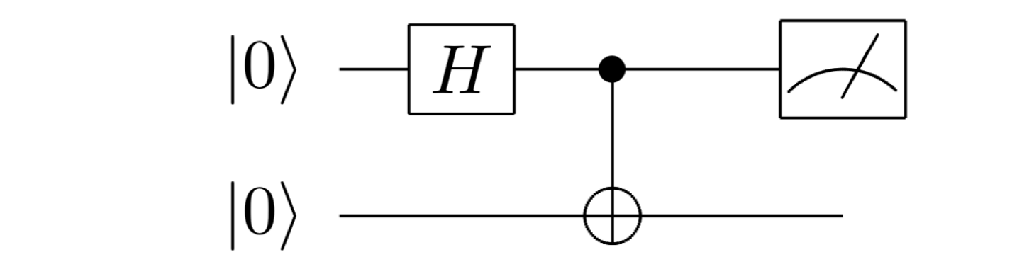
Hadamard Gate on the first qubit $ q_0 $: This gate places the qubit in a superposition of $ |0\rangle $ and $ |1\rangle $, enabling the representation of multiple states simultaneously.
CNOT Gate between $ q_0 $ (control) and $ q_1 $ (target): This entangles the two qubits. If $ q_0 $ is in the state $ |1\rangle $, the CNOT gate flips the state of $ q_1 $; otherwise, it leaves $ q_1 $ unchanged.
Measurement on $ q_0 $: Measures the state of $ q_0 $, collapsing the superposition to a definite state, either $ |0\rangle $ or $ |1\rangle $.

In this circuit, the combination of the Hadamard and CNOT gates creates an entangled state between $ q_0 $ and $ q_1 $. This setup is foundational for building more complex quantum algorithms, as entangled states are a key resource in quantum computing.

Quantum Algorithms in Data

Quantum Fourier Transform

The Quantum Fourier Transform (QFT) is the quantum analogue of the discrete Fourier transform, essential in quantum algorithms involving periodicity and phase estimation. The QFT maps an input state into the frequency domain, making it valuable for analyzing periodicity in quantum states and for applications in algorithms like Shor’s algorithm for factorization.

For an $ n $-qubit input state $ |x\rangle $, the QFT is defined as:

\[\begin{aligned} \text{QFT}|x\rangle = \frac{1}{2^{n/2}} \sum_{k=0}^{2^{n}-1} e^{2\pi i x k / 2^{n}} |k\rangle, \end{aligned}\]

where $ |x\rangle $ is an integer in the range $ 0 \leq x < 2^n $.

The QFT is constructed by applying a series of Hadamard gates and controlled phase rotations. For each qubit $ q_i $ (where $ i = 0, 1, \ldots, n-1 $), we perform a Hadamard transform followed by controlled rotations with angles depending on the separation of the qubits. This process creates a superposition that represents the Fourier transform of the input state.

For the $i$-th qubit in an $ n $-qubit system, the transformation steps are as follows:

Apply the Hadamard gate:
\[H |q_i\rangle = \frac{1}{\sqrt{2}} \left(|0\rangle + |1\rangle\right).\]
Follow with controlled rotations. For each pair $(i, j)$, where $ j > i $, apply a controlled-$R_k$ gate with rotation angle $ 2\pi / 2^{j-i+1} $:
\[R_k = \begin{bmatrix} 1 & 0 \\ 0 & e^{2\pi i / 2^k} \end{bmatrix}.\]
For instance, on the first qubit, this becomes:
\[H \cdot R_{k} = \frac{1}{\sqrt{2}} \left(|0\rangle + e^{2\pi i/2^k} |1\rangle \right),\]
where each controlled rotation $ R_k $ introduces a phase shift, creating interference patterns that encode the frequency information.
After applying all necessary gates, a swap gate sequence reorders the qubits to finalize the QFT computation in the correct order.

Example QFT Circuit for 3 Qubits

In a 3-qubit QFT circuit, the process involves:

Hadamard Gate on Qubit 0: Begin by placing qubit 0 in a superposition:
\[H|q_0\rangle = \frac{1}{\sqrt{2}} \left(|0\rangle + |1\rangle\right).\]
Controlled Rotations on Qubit 0: Apply controlled-$R_2$ and controlled-$R_3$ gates between qubit 0 and the subsequent qubits, introducing phases:
- Apply $R_2$ between qubit 0 and qubit 1.
- Apply $R_3$ between qubit 0 and qubit 2.
Hadamard Gate on Qubit 1: Apply a Hadamard gate to qubit 1 to further entangle it with the other qubits:
\[H|q_1\rangle = \frac{1}{\sqrt{2}} \left(|0\rangle + |1\rangle\right).\]
Controlled Rotation on Qubit 1: Apply a controlled-$R_2$ gate between qubit 1 and qubit 2.
Final Hadamard Gate on Qubit 2: Apply a Hadamard gate to qubit 2.
Swap Operation: To finalize, perform a swap between qubits 0 and 2 to ensure the qubits are in the correct order for measurement.

The resulting QFT circuit efficiently transforms the input state into the frequency domain, ready for analysis or further algorithmic steps.

Applications of the QFT include:

Signal Processing: The QFT accelerates Fourier transforms on large datasets, useful in applications requiring quantum frequency analysis, such as in signal processing within quantum data states.
Period Finding and Shor’s Algorithm: The QFT is critical in period-finding algorithms and enables efficient solutions to periodicity and factorization problems, a foundation for Shor’s algorithm in quantum cryptanalysis.

Grover’s Algorithm

Grover’s Algorithm provides a powerful quadratic speedup for unstructured search problems, reducing search complexity from $ O(N) $ to $ O(\sqrt{N}) $. This efficiency gain makes it particularly valuable for applications involving large datasets where specific items or optimal solutions need to be identified quickly. Grover’s approach relies on iteratively amplifying the probability amplitude of the target state, isolating it from other possible states through a process known as amplitude amplification.

The key to amplitude amplification in Grover’s Algorithm is the diffusion operator $ D $, which can be mathematically expressed as:

\[\begin{aligned} D = H^{\otimes n} \cdot \left( 2|0\rangle\langle0| - I \right) \cdot H^{\otimes n}, \end{aligned}\]

where $ H^{\otimes n} $ represents the Hadamard gate applied to each of the $ n $ qubits. This operator amplifies the target state’s probability by reflecting all states around their mean amplitude, boosting the likelihood of measuring the correct result.

Steps of Grover’s Algorithm

Initialization: Begin by initializing a superposition across all possible states:
\[|\psi\rangle = \frac{1}{\sqrt{N}} \sum_{x=0}^{N-1} |x\rangle\]
where each $ |x\rangle $ represents a potential solution.
Oracle Function $ O $: Use an oracle function to mark the target state by flipping its amplitude. Mathematically, this is represented as:
\[O|x\rangle = \begin{cases} -|x\rangle, & \text{if $x$ is the target} \\ |x\rangle, & \text{otherwise} \end{cases}\]
Amplitude Amplification (Diffusion): Following the oracle, apply the diffusion operator $ D $ to amplify the target state’s amplitude while suppressing others:
\[D = 2|\psi\rangle\langle\psi| - I,\]
where $ |\psi\rangle $ is the initial superposition. The operator $ D $ increases the probability of measuring the target state by reflecting all amplitudes about their average.
Iteration: Repeat the oracle and diffusion steps approximately $ \frac{\pi}{4}\sqrt{N} $ times to maximize the target state’s probability amplitude.
Measurement: Measure the quantum state to collapse it onto the target state with high probability.

Applications of Grover’s Algorithm

Database Search: Grover’s Algorithm provides a highly efficient search mechanism for unstructured datasets, making it ideal for quantum databases and systems where rapid data retrieval is essential.
Optimization Problems: In high-dimensional optimization tasks, Grover’s Algorithm can identify optimal solutions significantly faster than classical search methods, benefiting scenarios where conventional algorithms struggle with scalability.

Quantum Principal Component Analysis

Quantum PCA offers a quantum-enhanced approach to Principal Component Analysis (PCA), widely used for dimensionality reduction in machine learning and data engineering. By leveraging quantum computation, Quantum PCA can significantly accelerate the extraction of principal components, making it particularly advantageous for high-dimensional datasets.

The classical covariance matrix $ \Sigma $, which captures the variance structure of the data, can be approximated as a quantum density matrix $ \rho $ as follows:

\[\begin{aligned} \Sigma = \sum_{i=1}^{n} | x_i \rangle \langle x_i | \end{aligned}\]

where each data vector $ | x_i \rangle $ is represented as a quantum state. The density matrix $ \rho $, defined as:

\[\begin{aligned} \rho = \frac{1}{n} \sum_{i=1}^{n} | x_i \rangle \langle x_i |, \end{aligned}\]

serves as the quantum equivalent of the covariance matrix and allows for the representation of the dataset’s principal components.

The principal components are found by solving the eigenvalue problem for $ \rho $, where eigenvalues $ \lambda_i $ and eigenvectors $ | u_i \rangle $ satisfy:

\[\begin{aligned} \rho | u_i \rangle = \lambda_i | u_i \rangle. \end{aligned}\]

Using Quantum Phase Estimation (QPE), we can efficiently approximate the eigenvalues $ \lambda_i $ and their corresponding eigenvectors $ | u_i \rangle $.

Steps of Quantum PCA

Encoding the Covariance Matrix as a Quantum State

First, we represent the classical covariance matrix $ \Sigma $ of a dataset $ X \in \mathbb{R}^{n \times d} $ (where $ n $ is the number of observations and $ d $ is the number of features) as a quantum density matrix $ \rho $. Given by:
\[\begin{aligned} \Sigma = \frac{1}{n} X^T X, \end{aligned}\]
the matrix $ \Sigma $ is encoded as $ \rho $, a $ d \times d $ Hermitian matrix with similar properties to the covariance matrix. Quantum density matrix encoding leverages quantum states corresponding to each row of $ X $, capturing the structure of the data in the quantum realm.
Quantum Phase Estimation to Find Eigenvalues and Eigenvectors

To extract the principal components, we use Quantum Phase Estimation (QPE), which estimates the eigenvalues and eigenvectors of the density matrix $ \rho $. Through quantum parallelism, QPE simultaneously approximates multiple eigenvalues, yielding an eigenvalue decomposition of $ \rho $:
\[\begin{aligned} \rho = \sum_{i=1}^{d} \lambda_i | u_i \rangle \langle u_i |, \end{aligned}\]
where:
- $ \lambda_i $ represent the variance explained by each principal component,
- $ | u_i \rangle $ are the eigenvectors, or principal components.
The QPE algorithm applies a unitary transformation associated with $ \rho $ to a quantum register, allowing the quantum system to find eigenvalues and eigenvectors with high efficiency.
Measurement to Obtain Principal Components

After applying QPE, a measurement is performed, collapsing the quantum state onto the eigenvector corresponding to the largest eigenvalue, representing the primary principal component. Repeated measurements reveal the dominant principal components in order of explained variance, extracting key features without explicitly computing all eigenvalues and eigenvectors.

Applications of Quantum PCA

Significant Speedup: In classical PCA, the time complexity for diagonalizing a $ d \times d $ matrix is $ O(d^3) $, which is computationally expensive for large dimensions. Quantum PCA, leveraging Quantum Phase Estimation, reduces this to $ O(\log(d)) $, offering substantial speed improvements.
Efficiency in High-Dimensional Data: Quantum PCA processes data in a high-dimensional Hilbert space, making it possible to handle large datasets without the memory constraints typical of classical algorithms. By storing data as quantum states, the algorithm efficiently manages high-dimensional data with significantly reduced resources.

Potential Impact on Data Engineering

Quantum computing is set to transform data engineering by introducing efficient algorithms for high-dimensional data processing, machine learning, and secure data handling. Here’s how these potential impacts break down:

Speeding Up Data Processing

Quantum algorithms offer a promising speedup for data processing tasks, essential for managing petabyte-scale datasets.

Quantum Search Optimization: Algorithms like Grover’s Algorithm reduce search complexity from $O(N)$ to $O(\sqrt{N})$, making them ideal for rapid data retrieval in unstructured data sources.
Quantum Data Encoding: Encoding data using quantum states can provide efficient, scalable access to high-dimensional datasets, facilitating advanced ETL (Extract, Transform, Load) processes.

Enhancing Machine Learning Models

Quantum algorithms could accelerate model training and inferencing, boosting the performance of machine learning workflows in data engineering environments.

Quantum SVMs: Quantum-enhanced support vector machines utilize quantum kernels, offering exponential speedups over classical SVMs for high-dimensional classification tasks.

Quantum Kernel Function:
\[\begin{aligned} K(x_i, x_j) = |\langle \phi(x_i) | \phi(x_j) \rangle|^2, \end{aligned}\]
where $ |\phi(x)\rangle $ is the quantum feature map encoding data points into a quantum Hilbert space, improving separability for complex datasets.
Quantum Neural Networks (QNNs): QNNs provide quantum speedups for deep learning tasks, potentially enhancing the training times for applications like recommendation systems and anomaly detection.

Secure Data Transmission with Quantum Cryptography

Quantum cryptography introduces advanced security measures in data transmission, leveraging quantum mechanics for robust data encryption.

Quantum Key Distribution (QKD): QKD, particularly the BB84 Protocol, enables secure encryption by generating eavesdrop-resistant keys using quantum principles.
Quantum Secure Hashing: Quantum hashing algorithms can enhance the integrity of data transfers, ensuring that transmitted data remains tamper-proof during ETL workflows and across distributed data engineering environments.

Optimizing Data Pipelines and Scheduling

Optimization tasks are fundamental in data engineering, especially for resource allocation and scheduling. Quantum algorithms like quantum annealing can enhance pipeline scheduling and improve resource utilization.

Quantum Annealing for Task Scheduling: By solving complex combinatorial optimization problems, quantum annealing algorithms can streamline scheduling in distributed systems (like Spark clusters), improving efficiency across multiple ETL stages.
Network Path Optimization with Quantum Walks: Quantum walks accelerate network pathfinding, optimizing data transfer routes and reducing latency across distributed data nodes.

With these potential applications, quantum computing positions data engineers to innovate in data handling and machine learning processes. While full quantum capabilities are still emerging, familiarizing with these principles prepares data engineers to adopt quantum advancements as they mature.

Current Quantum Computing Platforms

A few leading platforms provide access to quantum computing resources, making it possible for data engineers and developers to experiment with quantum algorithms.

IBM Quantum Experience

Description: IBM Quantum Experience offers cloud-based access to IBM’s quantum processors, enabling users to run quantum experiments on actual quantum hardware. With over 20 quantum processors, IBM’s ecosystem provides one of the most accessible platforms for developers.
Tools: The platform utilizes Qiskit, a comprehensive, open-source quantum computing framework in Python that allows users to create, simulate, and execute quantum circuits.
Special Features: IBM Quantum Experience supports hybrid quantum-classical workflows, allowing developers to optimize and execute computations by combining classical and quantum resources.

Google Quantum AI

Description: Google Quantum AI focuses on advancing quantum hardware and developing quantum algorithms, with a strong research emphasis on achieving practical quantum advantage. Google’s quantum processors are designed to solve complex problems like optimization and machine learning tasks.
Tools: Cirq, a Python library provided by Google, allows developers to design and simulate quantum circuits specifically tailored to Google’s hardware. Cirq’s flexibility makes it suitable for customized experiments in quantum machine learning and optimization.
Special Features: Google Quantum AI is known for its breakthroughs in quantum supremacy and real-world applications in optimization, making it suitable for experimenting with data engineering tasks in high-dimensional spaces.

Microsoft Quantum

Description: Microsoft Quantum delivers a full-stack quantum computing ecosystem, including scalable quantum hardware, development tools, and a dedicated programming language, Q#. Microsoft’s platform aims to integrate quantum resources with Azure cloud services for seamless, scalable access.
Tools: Q# and the Quantum Development Kit (QDK) offer a robust environment for writing, simulating, and testing quantum algorithms. The QDK includes libraries for quantum machine learning, chemistry, and cryptography, supporting data engineering applications.
Special Features: The integration with Azure Quantum provides hybrid classical-quantum cloud workflows, enabling data engineers to combine quantum resources with Azure’s extensive data engineering and AI toolset for large-scale applications.

Amazon Braket

Description: Amazon Braket provides managed access to quantum hardware and simulators from leading quantum hardware providers, including Rigetti, D-Wave, and IonQ, via AWS. Braket offers a unified interface, making it easier for developers to experiment across multiple quantum processors.
Tools: Braket SDK, a Python library, supports the design and simulation of quantum circuits and annealing tasks directly within the AWS ecosystem. Braket’s integration with AWS services facilitates hybrid workflows.
Special Features: Amazon Braket provides scalability within the AWS ecosystem, allowing users to integrate quantum tasks with AWS’s storage, database, and machine learning services, making it highly adaptable for data engineering use cases.

Rigetti Quantum Cloud Services (QCS)

Description: Rigetti’s Quantum Cloud Services (QCS) platform provides access to Rigetti’s superconducting quantum processors and supports real-time integration with classical hardware, enabling faster, interactive experimentation.
Tools: Forest SDK and Quilc compiler (for the Quil language) provide tools for creating and executing quantum programs tailored to Rigetti’s quantum hardware.
Special Features: Rigetti’s emphasis on hybrid computation allows seamless classical-quantum integration, optimizing data engineering tasks that require both quantum processing and classical post-processing.

Getting Started with Quantum Computing

With quantum computing resources becoming more accessible, data engineers can begin to integrate quantum concepts and platforms into their workflows. Here are some practical steps to start working with quantum computing:

Understand Quantum Mechanics Basics: Begin with linear algebra, quantum states, and basic principles of quantum mechanics, as these are foundational to understanding quantum algorithms.
Learn Quantum Programming Languages: Explore Qiskit, Cirq, Q#, and Braket SDK, each of which provides unique features and access to various quantum hardware.
Experiment with Quantum Simulators: Quantum simulators on platforms like Qiskit and Cirq allow developers to test and debug quantum algorithms without requiring access to physical quantum hardware.
Implement Basic Quantum Algorithms: Begin with simple algorithms, such as Deutsch-Jozsa and Grover’s Algorithm, to gain a practical understanding of quantum principles.
Join Quantum Communities: Participate in online forums, workshops, and quantum hackathons. Engaging with the community can accelerate learning and provide opportunities to collaborate on quantum projects.

Conclusion

Quantum computing offers an unprecedented opportunity to reshape data engineering practices by introducing new dimensions of computational power through principles like superposition, entanglement, and quantum parallelism. As these concepts take shape in quantum algorithms such as Grover’s Algorithm and Quantum PCA, data engineers can begin to address limitations in classical computing, enabling faster search, retrieval, and dimensionality reduction in large datasets. This transformation holds significant promise for ETL workflows—where quantum-optimized search and data transformation could revolutionize data processing speeds, particularly when handling unstructured data in distributed environments like BigQuery and Elasticsearch.

The potential impact of quantum computing on machine learning is equally profound. Quantum-enhanced models, such as quantum SVMs and quantum neural networks, offer faster training times and improved accuracy, which are invaluable in applications like anomaly detection and real-time analysis. Quantum algorithms’ efficiency in handling high-dimensional feature spaces makes them ideal for the complex pattern recognition that big data environments demand.

Security, an increasingly critical component of data engineering, stands to benefit from quantum advancements as well. With quantum cryptographic protocols like Quantum Key Distribution (QKD), quantum computing introduces robust data encryption methods that address vulnerabilities in traditional security approaches. For data engineers responsible for sensitive data management across platforms like AWS and GCP, quantum cryptography could ensure data integrity and privacy, providing a future-proof security framework.

Quantum platforms such as IBM Quantum Experience, Google Quantum AI, and Amazon Braket now make it possible for data engineers to experiment with quantum algorithms within familiar cloud ecosystems. As these platforms mature, they will facilitate seamless hybrid workflows, blending quantum and classical resources, thus paving the way for practical applications of quantum computing in data engineering.

The evolving landscape of quantum software and developer tools like Qiskit, Cirq, and Braket SDK further lowers the barrier to entry, making it possible for data engineers to start working with quantum algorithms even without direct hardware access. As quantum capabilities continue to progress, future integration of quantum algorithms into data engineering workflows may become routine, with specialized tools and frameworks emerging to support this shift.

Although quantum computing remains in its formative stages, data engineers who build foundational quantum skills today will be well-positioned to adopt its applications as they become mainstream. With the potential to revolutionize data processing, elevate machine learning workflows, and secure data pipelines, quantum computing is on track to become indispensable in modern data engineering practices, making early adoption and readiness a strategic advantage for those aiming to stay at the cutting edge of technological innovation.