A first-order Markov chain process is characterized by the Markov property, which states that the conditional probability distribution for the system at the next time period depends only on the current state of the system, and not on the state of the system at any previous time periods.
A finite-state discrete-time Markov chain is a stochastic process that consists of a finite number of states and transition probabilities among the different states. The process evolves through successive time periods known as steps.
Definition: Discrete-time Markov Chain
Let a stochastic process $S = \{X_0, X_1, \cdots, X_n\}$ be a sequence of discrete random variables. Then the sequence $S$ is a Markov Chain if it satisfies the Markov property:
$$\begin{align}
\mathcal{P}(X_{t+1} = j | X_t = i, X_{t-1}, \cdots, X_1, X_0) &= \mathcal{P}(X_{t+1} = j | X_t = i) \nonumber \\
&= \mathcal{P}(X_{t} = j | X_{t-1} = i) \nonumber \\
&= \mathcal{P}(X_{1} = j | X_{0} = i) \ ,
\end{align}$$
for all $t=0,1,\cdots, n$ and all possible states $i, j = 1, \cdots, m$.
Thus, such a Markov chain process is memoryless. Consequently, it can be used for describing systems that follow a chain of linked events, where what happens next depends only on the current state of the system.
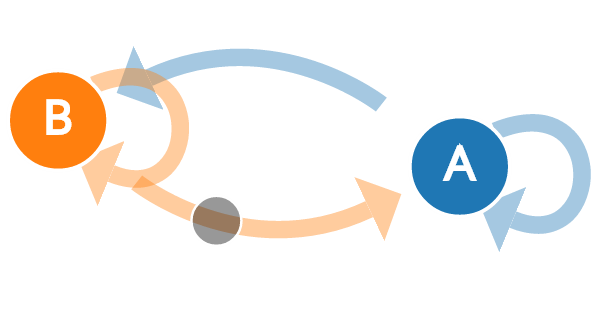 |
|---|
| A transition state diagram |
The Markov property is not merely sufficient for a process to be a Markov chain — it is the definition. A simple random walk, for instance, is a Markov chain precisely because its next position depends only on where it is now and not on the route it took to get there. What does exist are processes that fail the property as stated but satisfy a weakened version of it.
A Markov chain with memory (an order-$p$ chain) is a process satisfying,
\[\begin{align} \mathcal{P}(X_{t+1} = j | X_t = i, X_{t-1}, \cdots, X_1, X_0) = \mathcal{P}(X_{t+1} = j | X_t = i, X_{t-1}, \cdots, X_{n-p}) \nonumber \ , \end{align}\]for all $ n > p$. In this type of Markov chain, the future state depends on the past $p$ states where $p=1$ is equivalent to the usual Markov property.
A Markov chain is irreducible if there is a path from any state to any other state and aperiodic if the period of the chain is 1. A Markov chain is ergodic if it is both irreducible and aperiodic.
If the state space is finite, then the transition probability can be represented by a matrix $P$ whose $(i,j)$th element is given by:
\[\begin{align} P_{i j} = \mathcal{P}(X_{t+1} = j | X_t = i) \geq 0, \, \, \, \, \, \, \sum_{j=1}^m P_{i j} = 1 \ . \end{align}\]This matrix is also known as the one-step probability matrix, i.e. the $P_{i j}$ is the probability of moving from state $i$ to state $j$ in one-step in the chain. Similarly the $(i,j)$th element of the $k$-step probability matrix $P^{(k)}$ is,
\[\begin{align} P_{ij}^{(k)} &= \mathcal{P}(X_{t+k}=j | X_{t} = i) \ , \nonumber \\ &= \mathcal{P}(X_k = j | X_0 = i) \ , \nonumber \\ &\geq 0 \ , \end{align}\]and,
\[\begin{align} \sum_{j=1}^m P_{ij}^{(k)} = 1 \ , \, \, \, \text{ for }k = 0, \cdots, n \ . \end{align}\]This can be written in terms of the one-state transition matrix as $P_{ij}^{(k)} = (P^k)_{i j}$. As expected for $k=0,1$ we have,
\[\begin{align} P^{(0)} = I_m, \, \, \, \, P^{(1)} = P \ . \end{align}\]where $I_m$ is the $m \times m$ identity matrix and $P$ is the one-step transition matrix. The Chapman-Kolmogorov equation is,
\[\begin{align} P_{ij}^{(n)} = \sum_{\ell=1}^m P_{i \ell}^{(r)} P_{\ell j}^{(n-r)} \ , \qquad 0 \leq r \leq n \ , \end{align}\]where the sum runs over all $m$ states and $r$ is any intermediate step. This allows us to write the general property,
\[\begin{align} P^{(n + r)} = P^{(n)} P^{(r)} \ . \end{align}\]The steady state vector $\pi$ is defined as,
\[\begin{align} \lim_{n \rightarrow \infty} P_{ij}^{(n)} = \pi_j, \, \, \, \, \, \, \sum_{j=1}^m \pi_j = 1 \ . \end{align}\]We can determine this from the matrix equation,
\[\begin{align} \pi P = \pi \ . \end{align}\]The steady state vector is the eigenvector of $P$ with eigenvalue $1$. The steady state distribution is the probability distribution of the Markov chain at equilibrium and it is unique if the Markov chain is ergodic.
The expected number of steps to reach a given state $j$ from an initial state $i$ — the mean hitting time $k_{ij}$ — is not read off the powers of $P$ directly. It is the solution of a linear system obtained by conditioning on the first step:
\[\begin{align} k_{jj} = 0 \ , \qquad k_{ij} = 1 + \sum_{\ell \neq j} P_{i \ell} \, k_{\ell j} \quad \text{for } i \neq j \ . \end{align}\]In words: from any state other than the target, you spend one step and then find yourself at $\ell$ with probability $P_{i\ell}$, from where the expected remaining time is $k_{\ell j}$. Deleting row and column $j$ from $P$ to give $Q$, this is just
\[\begin{align} (I - Q) \, \vec{k} = \vec{1} \ , \end{align}\]a single linear solve. For an ergodic chain there is also a clean identity for the mean return time to a state, which is simply the reciprocal of its steady state probability:
\[\begin{align} k_{jj}^{\text{return}} = \frac{1}{\pi_j} \ . \end{align}\]Putting it together in code
The whole of the above is about twenty lines of NumPy. Consider a three-state weather chain — sunny, cloudy, rainy:
import numpy as np

states = ['sunny', 'cloudy', 'rainy']

P = np.array([
    [0.8, 0.15, 0.05],   # from sunny
    [0.3, 0.5,  0.2 ],   # from cloudy
    [0.2, 0.3,  0.5 ],   # from rainy
])

assert np.allclose(P.sum(axis=1), 1.0)      # rows must be distributions

# k-step transition matrix: P^(k) = P^k
P3 = np.linalg.matrix_power(P, 3)

# Steady state: the left eigenvector of P with eigenvalue 1, normalised.
eigenvalues, eigenvectors = np.linalg.eig(P.T)
stationary = np.real(eigenvectors[:, np.isclose(eigenvalues, 1)][:, 0])
stationary /= stationary.sum()
# -> array([0.567, 0.269, 0.164])

# Mean hitting times to state j: (I - Q) k = 1, with row/col j removed.
def mean_hitting_times(P: np.ndarray, target: int) -> np.ndarray:
    n = P.shape[0]
    keep = [i for i in range(n) if i != target]
    Q = P[np.ix_(keep, keep)]
    k = np.linalg.solve(np.eye(n - 1) - Q, np.ones(n - 1))
    out = np.zeros(n)
    out[keep] = k
    return out

# Mean return time to a state is 1 / pi_j.
return_times = 1 / stationary
Two things are worth noticing. Powering up $P$ converges to a matrix whose rows are all the stationary distribution — that is the definition of ergodicity made visible, and it is a good sanity check on any chain you fit. And the eigenvector route is exact where simulation would need millions of samples for the same precision.
Where this actually gets used
Markov chains are one of those pieces of undergraduate mathematics that turn out to be everywhere in applied work:
- Hidden Markov Models. The state is unobserved and you see only a noisy emission from it. Fitting an HMM to asset returns gives a regime — a probabilistic label for “we are currently in a low-volatility bull state” versus “we are in a crisis state” — with the transition matrix telling you how sticky each regime is. The persistence of the regimes is exactly the $P_{ii}$ entries, and the expected duration of a regime is $1/(1 - P_{ii})$.
- MCMC. The dominant method for Bayesian inference works by constructing a Markov chain whose stationary distribution is the posterior you want to sample from, then running it. Metropolis-Hastings and Gibbs sampling are both recipes for building a $P$ with a prescribed $\pi$ — a neat inversion of the problem posed in this post.
- PageRank. Google’s original ranking algorithm is the stationary distribution of a random surfer on the web graph, with a damping factor added specifically to make the chain irreducible and aperiodic so that $\pi$ exists and is unique.
- Reliability and queueing. System states (up, degraded, failed) with transition rates give expected time to failure directly from the hitting-time system above.
- Customer and credit modelling. Transition matrices between delinquency buckets are the standard tool for provisioning, and the $k$-step matrix is the forecast.
The common thread is that the modelling effort goes into choosing the state space. Get the states right and the memorylessness assumption is usually defensible; get them wrong and you end up with a chain that needs memory, at which point you either extend the state space — an order-$p$ chain over $m$ states is a first-order chain over $m^p$ composite states — or reach for a different model entirely.